Brownian bridges for stochastic chemical processes
Journal club presentation by Kyunghoon Han
Theoretical Chemical Physics Group, University of Luxembourg
Some facts on the paper
Title : Brownian bridges for stochastic chemical processes--An approximation method based on the asymptotic behavior of the backward Fokker-Planck equation
Authors : Shiyan Wang, Anirudh Venkatesh, Doraiswami Ramkrishna, Vivek Narsimhan of Purdue University
Their goal?
A fast approximation method to generate Brownian bridge process without solving the Backward Fokker-Planck (BFP) equation
The game plan
- Mathematical background
- Problem described by the authors
- Results and discussion
- Relevance to my work?
Brownian motion
A Brownian motion is described by what is called a Wiener process, $W_t$, parametrized by a variable $t$, which is defined as:- $W_0 = 0$
- $W_t-W_s \sim \mathcal{N}(0,t-s)$
- Each increment of $W_t$ is independent and is almost surely continuous
Brownian Bridge?
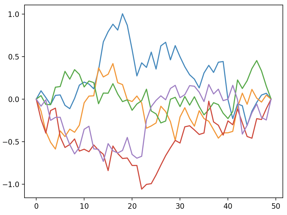
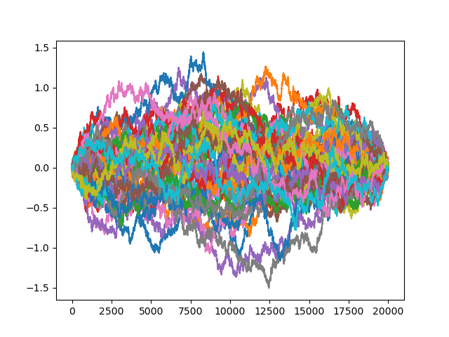
Suppose $(\mathcal{M},g)$ is a Riemannian manifold with $\dim\mathcal{M} = n$. If $X_t(s)$ is a Brownian motion defined on $(\mathcal{M},g)$, parametrized by a variable $t$ such that $X(0)=x\in\mathcal{M}$. The probability of finding $X_s(x)$ in some region $A\subset \mathcal{M}$, then, one may define: $$ \mathbb{P}\left\{X_s(x)\in A\right\} = \int_{\mathcal{M}} 1_{A}(z)p(s,x,z) \text{ vol}(dz) $$Simple simulation of a Brownian bridge
5 batches and 50 steps
10 batches and 100 steps

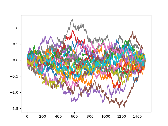
20 batches and 1500 steps
50 batches and 20000 steps
Stochastic D.E. in Itō form
Givens
- $s$ - a parameter of the path taken ($0 < s < L$)
- $\vec{x}(s)$ - position along the path
- drift term $\vec{A}$: the term that forces the position to change in some expected direction
- diffusion term $\vec{B}$: the random changes exerted on $\vec{x}$
Diffusion tensor: $D^{\mu\nu}=\frac{1}{2}B^\mu B^\nu$
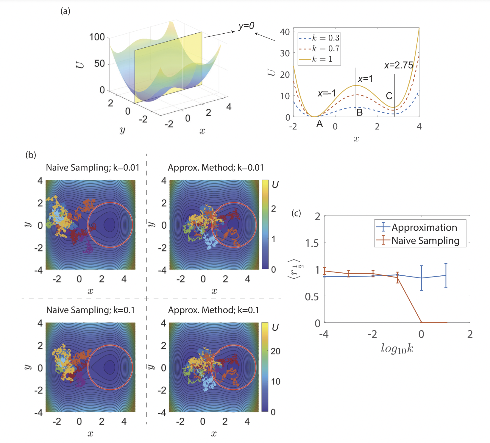
Example: Langevin equation
Suppose $\vec{A}=-ㄷ\nabla U$, $ㄷ$ a drift coefficient, for some continuous dimensionless external potential $U(\vec{x})$. Then the Itō's relation becomes: $$ d\vec{x} = ㄷ\cdot \nabla U ds +\vec{B}\sqrt{ds}\cdot \vec{Z} $$ where $\vec{Z} \sim \mathcal{N}^3(0,\vec{1})$.
Brownian bridge SDE?
An SDE that samples the conditional probability $P\left((\vec{s})|\vec{x}(0)=\vec{x}_0,\vec{x}(L)\in \Omega_L\right)$, i.e. a Brownian bridge $\vec{x}^{Br}$, is:
$$
d\vec{x}^{Br} = d\vec{x} + \underbrace{\vec{B}\vec{B}^T \frac{\partial}{\partial \vec{x}}\left(\ln q\right)}_{\text{additional drift}} ds
$$
with $\vec{x}(0)=\vec{x}_0$. Where...
Meaning that it is likely for the original random walk described by $d\vec{x}=\vec{A}ds + \vec{B} \cdot d\mathcal{B}$ to reach the target region, $\Omega_L$, at $s=L$.
The physical entropic free-energy barrier for reaching the end-state in $\Omega_L$ is proportional to $$ T\Delta S \sim -\beta \ln (q) $$
Computation of the hitting probability?
Assuming that $q$ is a probability associated to a Markov chain, the backward Fokker-Planck equation is: \[ \mathcal{L}^bq = \frac{\partial q}{\partial s} + \vec{A} \frac{\partial q}{\partial \vec{x}} + \frac{1}{2}\left(\vec{B}\vec{B}^T\right)\frac{\partial^2 q}{\partial \vec{x} \partial \vec{x}} \]Path integral approach?
the probability of attaining a specific path of the SDE $d\vec{x}=\vec{A}ds + \vec{B}\cdot d\mathcal{B}$ is expressed discretely as...$$ p\{\vec{x}\} \sim e^{-\frac{1}{2\Delta s}\sum_{k=0}^{N-1}\left(\Delta \vec{x}_k -\vec{A}\left(\vec{x}_k\right)\right)\cdot \left(\vec{B}\vec{B}^T\right)^{-1} \cdot \left(\Delta \vec{x}_k -\vec{A}\left(\vec{x}_k\right)\right)} $$ where $ \Delta \vec{x}_k = \vec{x}_{k+1}-\vec{x}_k$.
Reweighting
Instead of using $q$ as the hitting probability, consider an approximate hitting probability $\psi$.Ornstein-Uhlenbeck
$$ d\vec{x} = -k\vec{x}ds + \sigma d\mathcal{B} $$ for $k$ being the drift constant and $\sigma$ being the volatility of the random fluctuations.Geometric Brownian Motion
$$ d\vec{x} = k \vec{x}ds + \sigma \vec{x} d\mathcal{B} $$Result with Ornstein-Uhlenbeck
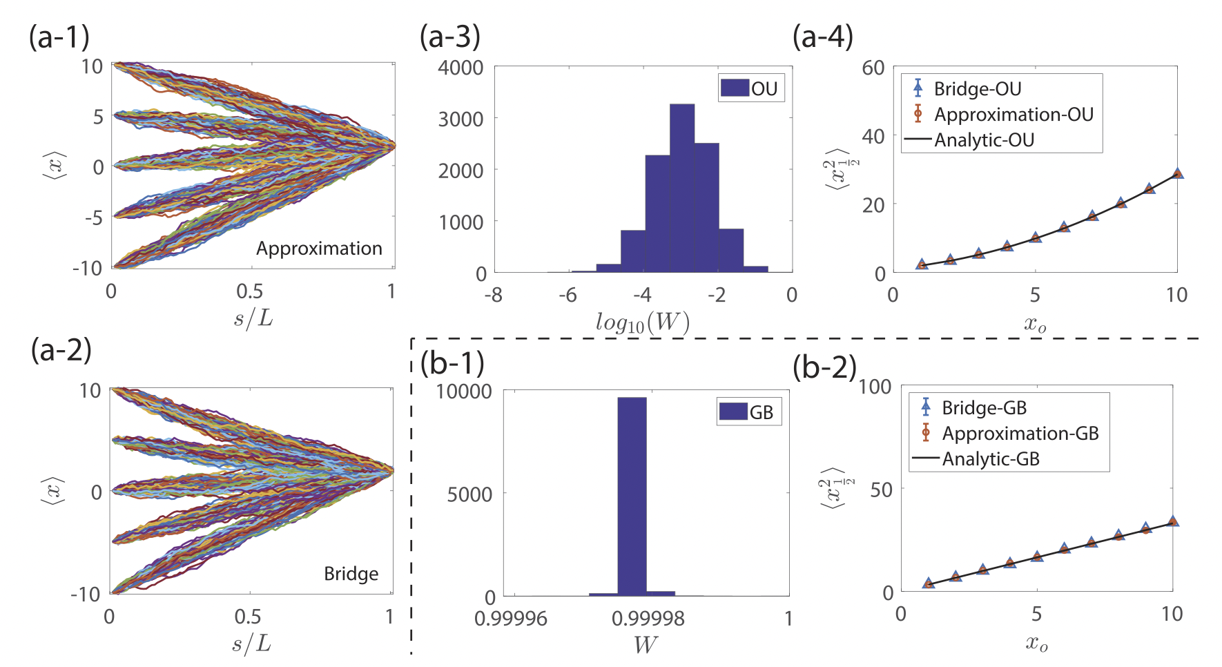
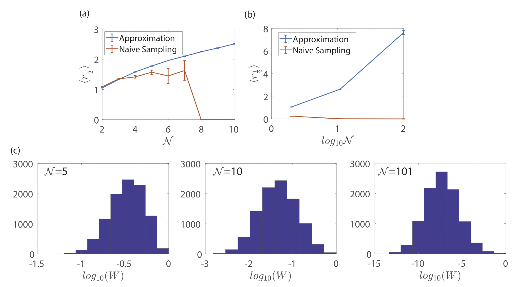
Normal bridge vs. introduced approximation
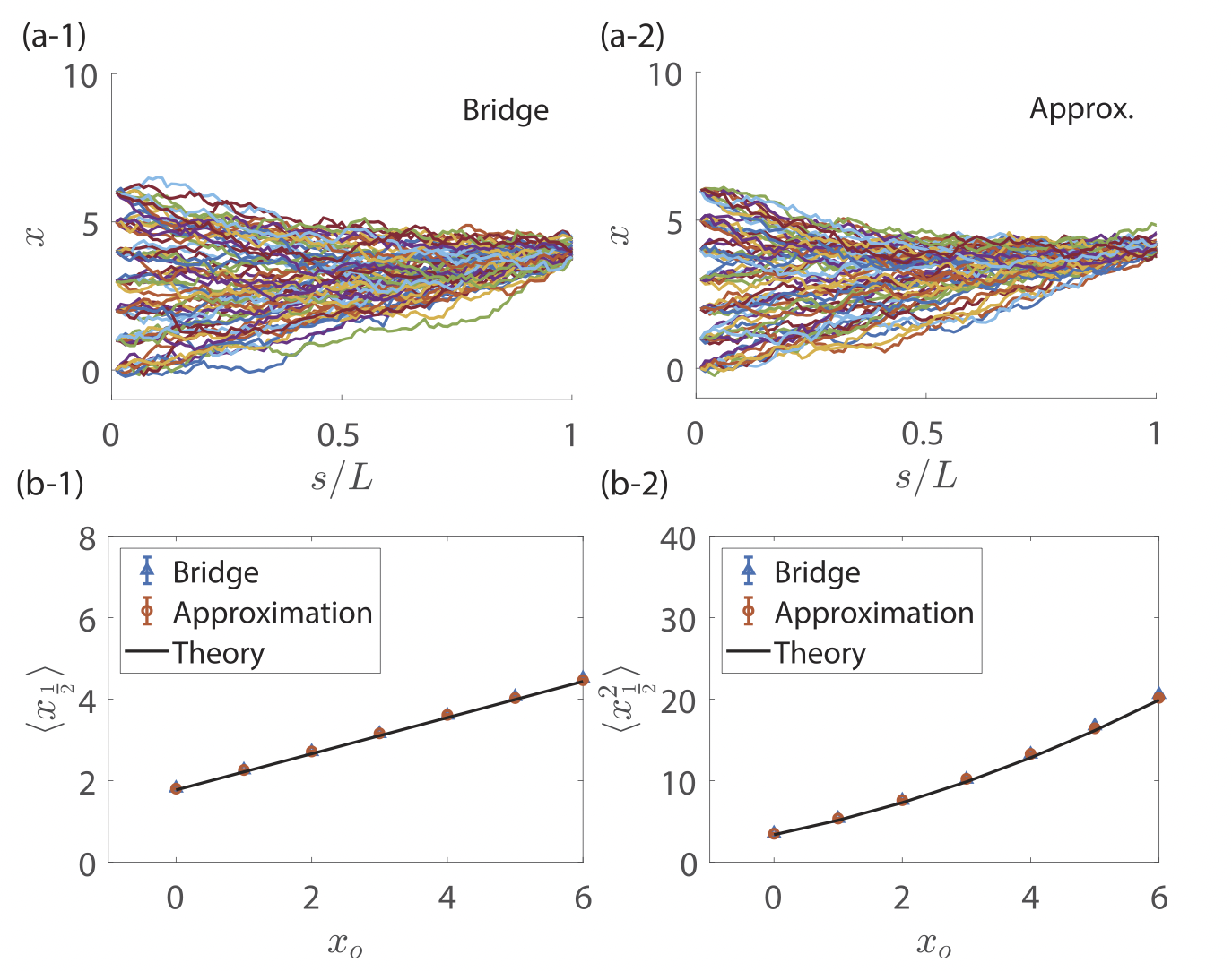
Naive sampling vs. introduced sampling