In a fairly recent paper published on ArXiv on 27th of December last year, Dr. Geoffrey Hinton¹ introduced a very interesting training algorithm that does not employ the backpropagation. Hinton, the father of backpropagation algorithm, explained in the introduction of the work that backpropagation remains implausible despite considerable effort to invent ways in which it could be implemented by real neurons¹ as our brain does not explicitly use the chain rule to update the parameters to learn something. Thus backpropagation is a poor choice of weight-update rule if one wants to simulate the way human brain learns.

In more practical side, Hinton mentions that

• backpropagation requires perfect knowledge of the forward-pass,
• reinforcement learning scales badly, and forward-forward (FF) algorithm may be a good alternative if the forward computations are not exactly known by construction.

My interest on this algorithm is whether we can have an exact mathematical representation of the data learned by a network of interest using the FF algorithm.

The idea

The FF algorithm replaces the forward and backward passes by two forward passes. One forward pass would take what Hinton calls a positive data and another forward pass would take a negative data. The positive forward pass, respectivly negative forward pass, will update its weight according to the positive, respectively negative, data it takes. Essentially, the positive data are real data to train on where the negative data are fake or perturbed data where its individual datum resembles the real data in some manner. Note that the negative data are not simple noise input.

To define the nature of positive and negative data, one needs to define what it means by goodness.

Definition 1 (Goodness) Let \(\ell\) be a neural network layer such that \(\ell : \mathcal{M}\rightarrow \mathcal{N}\) where \(\mathcal{M}\) and \(\mathcal{N}\) are manifolds where input and output vectors live, respectively. Let \(\mu : \mathcal{N} \rightarrow \mathbb{R}\) be a convex continuous non-negative function and \(\theta\) be a real positive number. The Goodness, \(G\), is then defined as \[G(m) = \sigma \left( \mu \left( \ell \left(m\right) - \theta \right)\right)\]

where \(\sigma\) is a logistics function.

The threshold \(\theta\) is chosen to ensure that the so-called positive data, i.e. the real data, will have positive goodness and the negative data will have negative goodness.

How to construct the negative data?

Hinton does not provide a general, canonical algorithm to show how to construct a negative data for any dataset. However, for MNIST data, he does show exactly how he created the negative dataset for his model. His recipe was:

1. mask the input real, i.e. positive, data,
2. mask another real data,
3. compose the two masked data.

The procedure is very well-illustrated from a figure from Hinton’s paper: 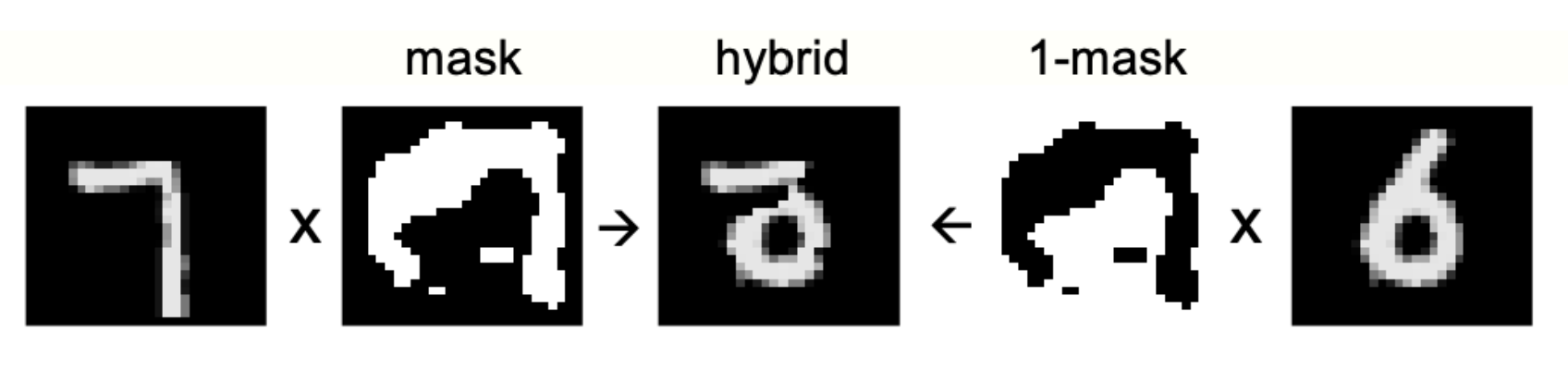Note that the resulting negative data resembles a data from MNIST dataset, but does not correspond to any of the integers one wishes to train on.

Another remark Hinton makes in both the paper and through the interview with Eye on AI² on negative data is to use the result from the model itself as its negative data–as done in training a Boltzmann machine.

Formulation / training algorithm

Say one’s interested in training a deep FF neural network with \(r\)-layers. This will then imply that for each layer, \(j\), one will have the corresponding goodness \(G_j\). Training \(j\)-th layer would have two phases per step: positive and negative training phases.

In the positive training phase of step \(i\) of the layer \(j\), we first compute \(s_j = G_j\left( \mathbf{W}_j \left(\mathbf{x}_{j-1}\right) \right)\) where \(\mathbf{W}_{j$}\) stands for a map that takes the output of the previous layer, \(\mathbf{x}_{j-1}\), to the output of the layer \(j\). The goal of the positive phase is to improve the score given by the goodness. This will evoke an optimisation problem that drives the goodness to be as large as possible, i.e. a problem of achieving \(\min \left\{ {s_j}^2 - {G_j}^2\right\}\).

In the negative training phase of step \(i\) of the layer \(j\), we take a negative input \(\mathbf{x}^n_{j-1}\) to compute the goodness as \(n_j = G_j \left( \mathbf{W}_j \left(\mathbf{x}^n_{j-1}\right) \right)\) and solve an optimisation problem where \(n_j\) is as small as possible, i.e. we want to force \(n_j \rightarrow 0\).

Notes on \(n_j\) and \(s_j\)

In attempts to unlearn the goodness of the perturbed or negative data, more nodes of the network will take part in each learning attempt. I did not see any mathematical proof on this statement yet. However, intuitively speaking, as the neurons are forced to learn the odd-patterns after being trained on a set of good inputs they would be guided/updated to seek more possibilities to understand the nature of the problem.

Embarrassing remark

Hinton mentions of a way to reformulate the above so that the algorithm somewhat recovers the benefits of the backpropagation algorithm by somehow transforming the architecture to resemble an RNN model. I could not understand the details of such transformation / algorithm at the moment.

Hopefully I can soon…

Anyhow, I shall write on my implementation of the FF algorithm in the part II of the article sometime soon.