Please note that the material below is written for the first year physics students enrolled in Programming for Physics (BA_PHYS_GEN-30) offered by the Department of Physics and Materials Science, University of Luxembourg.

1-dimensional Laplace equation

The 1D Laplace equation of a function ϕ:ℝ→ℝ is defined as \[\frac{d^2\phi}{dx^2} =0.\]

Integrating the both sides twice yields the solution of the form \[\phi(x) = \alpha x + \beta\]

where α and β are integration constants.

In physics, this equation is often called a heat equation as the equation is often used to examine the heat flow between two locations with different temperature readings.

Say, at x=0, the thermometer reads 25°C and the same thermometer records 45°C at x=10. The integration constants, in this case, are β=25 and α=2.

Numerical approximation of second derivative

Note that one can define the first derivative of ϕ as \[\frac{d\phi}{dx} = \lim_{h\rightarrow 0}\frac{\phi(x+h/2) - \phi(x-h/2)}{h}.\]

This immeidately allows us to write the second derivative of ϕ as \[\frac{d^2\phi}{dx^2} = \lim_{k,h,l\rightarrow 0} \frac{\frac{\phi(x+k/2+h/2) - \phi(x+k/2-h/2)}{h} - \frac{\phi(x-k/2+l/2) - \phi(x-k/2-l/2)}{l}}{k}.\]

Noting that the dummy variables for the limit are chosen arbitrarily, one can immediately show that the above equation can be rewritten as \[\frac{d^2\phi}{dx^2} = \lim_{h\rightarrow 0} \frac{\phi(x+h)+\phi(x-h) - 2\phi(x)}{h^2}.\]

This implies that if one wants to numerically compute the second derivative at point x, one must take three points: x-Δx, x, x+Δx. Say all the independent variables used to solve the equation are given in vector format as \[\mathbf{x} = \left[x_0, x_1, \cdots, x_{n-1}, x_n\right]^T.\]

The second derivative of ϕ, then, can be written as \[\frac{d^2\phi(\mathbf{x})}{d\mathbf{x}^2} = D\phi(\mathbf{x})\]

where \[D = \left[ {D_0}^T, {D_1}^T , \cdots {D_i}^T , \cdots , {D_n}^T \right]^T\]

with \[D_i = \left[ 0, 0, \cdots, 0, 1, -2, 1, 0, \cdots, 0 \right]\]

where the -2 is located at the i-th entry of the vector Dᵢ.

Numerical solution of the 1D Laplace equation

Note that the 1D Laplace equation essentially requires the following to hold \[\frac{\phi(x+h) + \phi(x-h) - 2\phi(x)}{h^2} \rightarrow 0\]

as the step-size goes to zero. As the step-size is never zero, the above limit implies that essentially we are trying to achieve \[\phi(x) \approx 0.5 (\phi(x+\Delta x) + \phi(x-\Delta x)).\]

In a numerical simulation, this process can be repeated until the difference between the n-th (ϕⁿ) and (n-1)-th solution (ϕⁿ⁻¹) is less than some very small threshold (say 10⁻¹²).

The answer can be verified by numerically differentiating the n-th solution twice (call this derivative ϕⁿ°) and examine the difference between ϕⁿ° and 0. One may use this difference as the threshold to decide when the algorithm should terminate. The next section introduces how one may obtain ϕⁿ°.

Extension to 3-dimensions

The above analysis can be applied to a three-dimensional Laplace equation: \[\nabla^2 \phi = \frac{\partial^2 \phi}{\partial x^2}+\frac{\partial^2 \phi}{\partial y^2}+\frac{\partial^2 \phi}{\partial z^2} = 0\]

by applying the above method in x, y and z-directions separately. Then you can obtain a nice picture like the one shown below!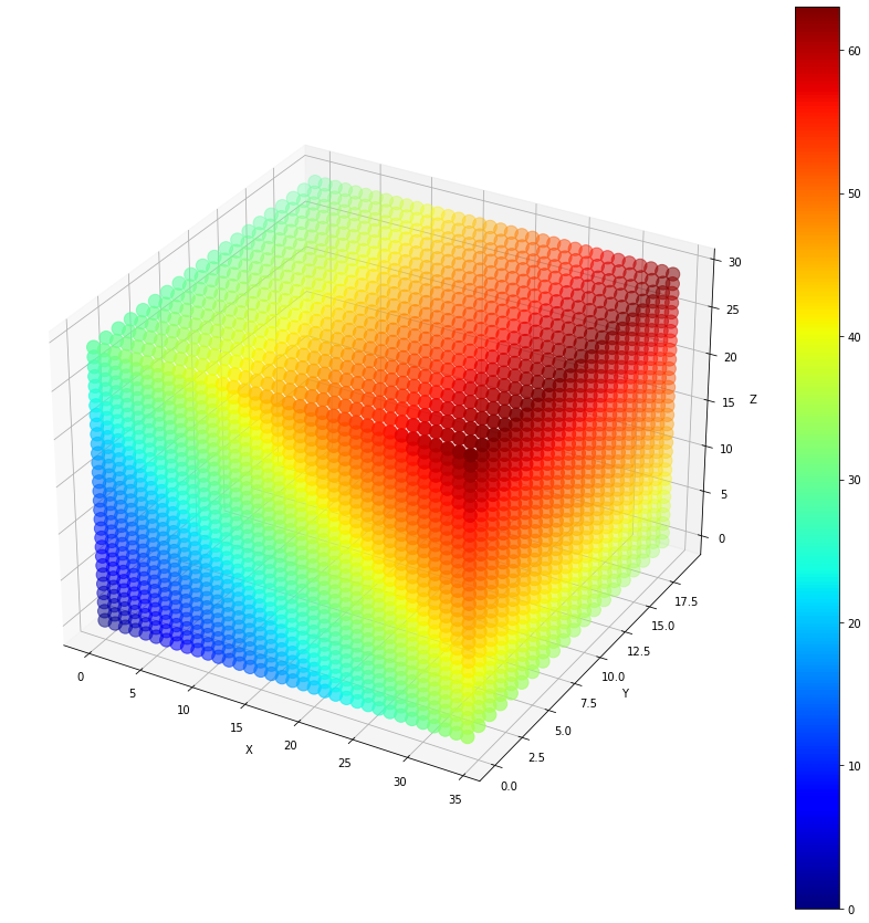

1D Wave Equation

A one-dimensional wave equation takes the form \[c^2 \frac{\partial^2 \phi}{\partial x^2} = \frac{\partial^2 \phi}{\partial t^2}.\]

Note that as ϕ now depends on both time and position, it needs both initial and boundary conditions.

Discretizing the wave equation

Let ϕⁱⱼ be the value of ϕ at i-th time measurement and j-th position measurement. If x is measured at j-th position measurement, x+Δx is registered at the (j+1)-th measurement. Similarly, if t is measured at i-th time measurement, t+Δt is registered at the (i+1)-th measurement.

First, to numerically compute the spatial second derivative of ϕ, fix the time-measurement index (i.e. the superscript i is fixed for now). By applying the method introduced above, one can immediately see that \[\frac{\partial^2 \phi^i(x)}{\partial x^2} = \frac{\phi^i(x+\Delta x)+\phi^i(x-\Delta x) - 2\phi^i(x)}{\Delta x^2}.\]

Thus, \[\frac{\partial^2 \phi^i_j}{\partial x^2} = \frac{\phi^i_{j+1} + \phi^i_{j-1} - 2\phi^i_j}{\Delta x^2}\]

holds.

Similarly, the second-derivative in time can be written as \(\frac{\partial^2 \phi^i_j}{\partial t^2} = \frac{\phi^{i+1}_j + \phi^{i-1}_j - 2\phi^i_j}{\Delta t^2}\)

The wave equation, then, becomes \[c^2\frac{\phi^i_{j+1} + \phi^i_{j-1} - 2\phi^i_j}{\Delta x^2} = \frac{\phi^{i+1}_j + \phi^{i-1}_j - 2\phi^i_j}{\Delta t^2}\]

which can be rearranged to the following recursive formula \[\phi^{i+1}_j = 2\phi^i_j - \phi^{i-1}_j + \frac{c^2\Delta t^2}{\Delta x^2}K^i_j\]

where \[K^i_j = \phi^i_{j+1}+ \phi^i_{j-1}-2\phi^i_j.\]

Note that the initial conditions are rather tricky to find. The Taylor approximation to the first order may be written as \(\phi_j(t+ \Delta t) \approx \phi(t) + \frac{\partial \phi}{\partial t}\Delta t\) and \(\phi_j(t- \Delta t) \approx \phi(t) - \frac{\partial \phi}{\partial t}\Delta t.\)

Subtracting one from the other, the following result is immediately derived: \(\frac{\partial \phi_j}{\partial t} = \frac{\phi_j(t+\Delta t)-\phi_j(t-\Delta t)}{2\Delta t} = W\) where W is the initial condition asserted on the first time derivative. Thus, the initial condition can be recursively defined as \(\phi^{i-1}_j = \phi^{i+1}_j + 2\Delta t W\)